Fitting Emax models for continuous outcomes • emaxnls

library(emaxnls)
library(tibble)
library(ggplot2)
theme_set(theme_bw())
set.seed(123)

This article walks through the process of fitting an Emax regression model to a continuous outcome with emax_nls(). It describes the model that is being fitted, sets out the estimation problem that emax_nls() solves under the hood, and then works through how to read and interpret the outputs. Binary outcomes follow a slightly different logic — they are fitted with emax_logistic() on the logit scale using iterative reweighted least squares — and are covered in a separate article.

The Emax model

The Emax model is a widely used exposure-response model in pharmacometrics. It describes a smooth, saturating relationship between a measure of drug exposure (a dose, a concentration, an AUC) and a response. As exposure increases the response moves away from a baseline value and asymptotes towards a maximal effect. The appeal of the model is that its parameters have direct pharmacological meaning.

The hyperbolic Emax function

In its basic (hyperbolic) form, the expected response $y$ at exposure $x$ is

$y = E_0 + E_{\max}\,\frac{x}{x + EC_{50}}.$

The three structural parameters are:

$E_0$ — the baseline response, i.e. the expected response at zero exposure ( $x = 0$ ). This is the placebo or pre-treatment level.
$E_{\max}$ — the maximal effect, the largest change from baseline that the drug can produce. As $x \to \infty$ the response approaches $E_0 + E_{\max}$ .
$EC_{50}$ — the exposure that produces half of the maximal effect. When $x = EC_{50}$ the term $x / (x + EC_{50}) = 1/2$ , so the response is exactly halfway between $E_0$ and $E_0 + E_{\max}$ . It is a measure of potency: a smaller $EC_{50}$ means the drug reaches its effect at lower exposures.

Because $EC_{50}$ is a strictly positive quantity that often spans several orders of magnitude, the package estimates it on the log scale. Internally the model works with $\log EC_{50}$ , which keeps the parameter unconstrained and tends to make the optimisation better behaved. This is why the parameter is named logEC50 throughout the interface.

The sigmoidal (Hill) extension

The hyperbolic model can be generalised by adding a Hill coefficient $h$ , which controls the steepness of the curve:

$y = E_0 + E_{\max}\,\frac{x^{h}}{x^{h} + EC_{50}^{\,h}}.$

When $h = 1$ this reduces to the hyperbolic model. Larger values of $h$ produce a steeper, more switch-like response. Like $EC_{50}$ , the Hill coefficient is positive and is estimated on the log scale as logHill. A sigmoidal model is requested by including a logHill term in the covariate model (see below); without it, emax_nls() fits the hyperbolic model.

Adding covariates

In practice the structural parameters often depend on subject-level characteristics: baseline severity might shift $E_0$ , body weight might modify $E_{\max}$ , and so on. In this package each structural parameter is given its own linear submodel. For example, allowing a continuous covariate to act on the baseline,

$E_0 = \beta_{0}^{E_0} + \beta_{1}^{E_0}\, z,$

means that the baseline response is itself a linear function of the covariate $z$ . Each structural parameter ( $E_0$ , $E_{\max}$ , $\log EC_{50}$ , and optionally $\log \text{Hill}$ ) can carry its own covariates in the same way. The intercept terms are the values the parameter takes when all covariates are zero.

You specify these submodels with a list of two-sided formulas passed to the covariate_model argument. A formula like E0 ~ age + group puts age and group on the baseline, while Emax ~ 1 says “estimate a single intercept, no covariates” for the maximal effect. At a minimum you must supply formulas for E0, Emax, and logEC50.

The example data

The package ships with a synthetic dataset, emax_df, that we use throughout. It is entirely simulated, which is convenient here because we know the true data-generating parameters and can check the estimates against them.

emax_df
#> # A tibble: 400 × 12
#>       id  dose  exp_1  exp_2 rsp_1 rsp_2 cnt_a cnt_b cnt_c bin_d bin_e cat_f
#>    <int> <dbl>  <dbl>  <dbl> <dbl> <dbl> <dbl> <dbl> <dbl> <dbl> <dbl> <fct>
#>  1     1   200 12332. 13004. 15.7      1  3.85  5.89  4.31     1     1 grp 1
#>  2     2   300 18232. 17244. 15.3      1  4.78  7.25  3.73     1     1 grp 1
#>  3     3     0     0      0   5.65     0  1.22  9.24  2.41     1     1 grp 1
#>  4     4   200  9394.  8839. 12.5      0  2.68  7.14  3.76     1     1 grp 2
#>  5     5   200  7088.  9827. 13.2      1  4.27  5.57  9.05     0     1 grp 2
#>  6     6   300 30402. 28483. 16.8      1  6.09  6.08  4.62     0     1 grp 1
#>  7     7   300 21679. 17137. 17.4      1  7.5   8.1   2.08     0     1 grp 3
#>  8     8   100 15506. 13377. 15.9      0  3.65  6.89  3.56     0     1 grp 1
#>  9     9     0     0      0   7.3      0  4.84  3.77  7.44     0     1 grp 2
#> 10    10   200  5331.  5251. 12.8      1  4.45  3.42  1.66     1     0 grp 3
#> # ℹ 390 more rows

The columns we care about for a continuous-outcome analysis are:

exp_1 — an exposure variable (there is a correlated second exposure metric, exp_2),
rsp_1 — the continuous response,
cnt_a, cnt_b, cnt_c — continuous covariates,
bin_d, bin_e — binary covariates,
cat_f — a categorical covariate.

The continuous response rsp_1 was generated from a hyperbolic Emax model with $E_0 = 5$ , $E_{\max} = 10$ , and $EC_{50} = 4000$ (so $\log EC_{50} \approx 8.29$ ), Gaussian noise with standard deviation $0.5$ , and a genuine effect of cnt_a on the baseline (a coefficient of $0.5$ ). The other covariates have no true effect. A good fit should recover these values, which gives us something concrete to look for when we interpret the output.

A quick look at the raw exposure-response relationship shows the characteristic Emax shape — a rise from baseline that flattens out at higher exposures:

ggplot(emax_df, aes(exp_1, rsp_1)) +
  geom_point(alpha = 0.3) +
  labs(x = "Exposure (exp_1)", y = "Response (rsp_1)")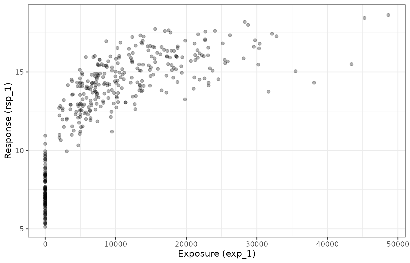

The estimation problem

Given the structural and covariate models, fitting reduces to finding the parameter values that make the predicted responses as close as possible to the observed responses. Writing $f(x_i, z_i; \theta)$ for the Emax prediction at the $i$ -th observation and $\theta$ for the full vector of coefficients, emax_nls() solves the nonlinear least squares problem

$\hat{\theta} = \arg\min_{\theta} \sum_{i=1}^{n} \big(y_i - f(x_i, z_i; \theta)\big)^2 .$

Under the usual assumption of independent, normally distributed errors with constant variance, this least squares solution is also the maximum likelihood estimate. (If you supply a weights vector via emax_nls_options(), the package minimises the weighted sum of squares instead.)

Two features make this harder than ordinary linear regression:

It is nonlinear. The prediction $f$ is not a linear function of the parameters (the exposure enters through $x / (x + EC_{50})$ ), so there is no closed-form solution. The estimate is found by iterative optimisation.
It needs starting values. Iterative optimisers must be given an initial guess for every parameter, and for nonlinear models a poor guess can lead to non-convergence or a local optimum.

Starting values

You rarely need to construct starting values by hand. emax_nls() calls emax_nls_init(), which uses data-driven heuristics — fitting a crude log-linear model to the dosed observations, reading off a baseline from the placebo records, and so on — to produce sensible starting values, together with lower and upper bounds for bounded optimisation. You can inspect what it comes up with:

emax_nls_init(
  structural_model = rsp_1 ~ exp_1,
  covariate_model = list(E0 ~ cnt_a, Emax ~ 1, logEC50 ~ 1),
  data = emax_df
)
#> # A tibble: 4 × 5
#>   parameter covariate start  lower upper
#>   <chr>     <chr>     <dbl>  <dbl> <dbl>
#> 1 E0        cnt_a      0    -7.84   7.84
#> 2 E0        Intercept  9.73  0.528 18.9 
#> 3 Emax      Intercept  7.74 -1.47  16.9 
#> 4 logEC50   Intercept  8.69  6.63  10.8

The parameter and covariate columns identify each coefficient, start is the initial guess, and lower/upper are the bounds used when a bounded algorithm is selected.

Choosing an optimiser

The optimisation algorithm and other fitting controls are set with emax_nls_options(), whose result is passed to the opts argument of emax_nls(). Three algorithms are supported:

"gauss" (the default) — the Gauss-Newton algorithm, equivalent to the default method in stats::nls().
"port" — bounded optimisation using the nl2sol routine from the PORT library. This respects the lower/upper bounds and is useful when parameters must stay within a plausible range.
"levenberg" — the Levenberg-Marquardt algorithm via minpack.lm::nlsLM(), which is often more robust when starting values are poor.

emax_nls_options()
#> $optim_method
#> [1] "gauss"
#> 
#> $optim_control
#> $optim_control$maxiter
#> [1] 50
#> 
#> $optim_control$tol
#> [1] 1e-05
#> 
#> $optim_control$minFactor
#> [1] 0.0009766
#> 
#> $optim_control$printEval
#> [1] FALSE
#> 
#> $optim_control$warnOnly
#> [1] FALSE
#> 
#> $optim_control$scaleOffset
#> [1] 0
#> 
#> $optim_control$nDcentral
#> [1] FALSE
#> 
#> 
#> $quiet
#> [1] FALSE
#> 
#> $weights
#> NULL
#> 
#> $na.action
#> function (object, ...) 
#> UseMethod("na.omit")
#> <bytecode: 0x563407999288>
#> <environment: namespace:stats>
#> 
#> $max_time
#> [1] Inf

Fitting the model

With the pieces in place, fitting the model is a single call. We specify the structural_model (response and exposure), the covariate_model (a submodel for each structural parameter), and the data:

mod <- emax_nls(
  structural_model = rsp_1 ~ exp_1,
  covariate_model = list(
    E0 ~ cnt_a,   # allow the baseline to depend on cnt_a
    Emax ~ 1,     # single intercept for the maximal effect
    logEC50 ~ 1   # single intercept for log-EC50
  ),
  data = emax_df
)

Before doing anything with a fitted object it is worth confirming that the optimiser converged. If it did not, most methods return a placeholder rather than misleading numbers:

emax_converged(mod)
#> [1] TRUE

Printing the object gives a compact summary: the structural model, the covariate submodels, the model type (hyperbolic or sigmoidal), and a coefficient table.

mod
#> Structural model:
#> 
#>   Exposure:       exp_1 
#>   Response:       rsp_1 
#>   Emax type:      hyperbolic 
#>   Response type:  continuous
#> 
#> Covariate model:
#> 
#>   E0:       E0 ~ cnt_a 
#>   Emax:     Emax ~ 1 
#>   logEC50:  logEC50 ~ 1 
#> 
#> Model fit:
#> 
#>   Observations:         400 
#>   Residual df:          396 
#>   Residual std. error:  0.5108 
#>   AIC:                  603.6 
#> 
#> Coefficients (95% CI):
#> 
#>   label             estimate std_error lower  upper
#> 1 E0_cnt_a             0.486    0.0116 0.463  0.509
#> 2 E0_Intercept         5.05     0.0759 4.91   5.20 
#> 3 Emax_Intercept       9.97     0.112  9.75  10.2  
#> 4 logEC50_Intercept    8.27     0.0394 8.19   8.35 
#> 
#> Use summary() for hypothesis tests.

Interpreting the output

Coefficients

The fitted coefficients are extracted with coef(). Each name encodes a structural parameter and a term: E0_Intercept is the baseline intercept, E0_cnt_a is the slope of the baseline on cnt_a, Emax_Intercept is the maximal effect, and logEC50_Intercept is log-EC50.

coef(mod)
#>          E0_cnt_a      E0_Intercept    Emax_Intercept logEC50_Intercept 
#>            0.4861            5.0548            9.9697            8.2688

Reading these against the known truth: E0_Intercept should be near $5$ , E0_cnt_a near $0.5$ , Emax_Intercept near $10$ , and logEC50_Intercept near $\log(4000) \approx 8.29$ .

Because logEC50 (and logHill, if present) are estimated on the log scale, their raw coefficients are not on the most interpretable units. Setting back_transform = TRUE exponentiates them and drops the log prefix, so logEC50_Intercept becomes EC50_Intercept on the exposure scale:

coef(mod, back_transform = TRUE)
#>       E0_cnt_a   E0_Intercept Emax_Intercept EC50_Intercept 
#>         0.4861         5.0548         9.9697      3900.4237

The back-transformed $EC_{50}$ should land near the true value of $4000$ .

Standard errors, tests, and confidence intervals

summary() returns a tidy coefficient table combining the estimate, its standard error, a $t$ -statistic and $p$ -value (testing whether the coefficient differs from zero), and a confidence interval.

summary(mod)
#> # A tibble: 4 × 7
#>   label             estimate std_error t_statistic    p_value ci_lower ci_upper
#>   <chr>                <dbl>     <dbl>       <dbl>      <dbl>    <dbl>    <dbl>
#> 1 E0_cnt_a             0.486    0.0116        42.1  3.63e-148    0.463    0.509
#> 2 E0_Intercept         5.05     0.0759        66.6  4.16e-217    4.91     5.20 
#> 3 Emax_Intercept       9.97     0.112         89.3  2.11e-264    9.75    10.2  
#> 4 logEC50_Intercept    8.27     0.0394        NA   NA            8.19     8.35

The $p$ -value for E0_cnt_a should be small, reflecting the real covariate effect built into the data, whereas a covariate with no true effect would show a large $p$ -value and an interval straddling zero. The back_transform and conf_level arguments work here too:

summary(mod, conf_level = 0.99, back_transform = TRUE)
#> # A tibble: 4 × 7
#>   label          estimate std_error t_statistic    p_value ci_lower ci_upper
#>   <chr>             <dbl>     <dbl>       <dbl>      <dbl>    <dbl>    <dbl>
#> 1 E0_cnt_a          0.486    0.0116        42.1  3.63e-148    0.456    0.516
#> 2 E0_Intercept      5.05     0.0759        66.6  4.16e-217    4.86     5.25 
#> 3 Emax_Intercept    9.97     0.112         89.3  2.11e-264    9.68    10.3  
#> 4 EC50_Intercept 3900.      NA             NA   NA         3519.    4313.

For confidence intervals on their own, confint() computes profile likelihood intervals rather than simple Wald (estimate $\pm$ 2 SE) intervals. Profile intervals are generally preferred for nonlinear models because they do not assume the likelihood surface is quadratic around the estimate, so they can be asymmetric:

confint(mod)
#>                     2.5%   97.5%
#> E0_cnt_a          0.4634  0.5089
#> E0_Intercept      4.9055  5.2041
#> Emax_Intercept    9.7525 10.1915
#> logEC50_Intercept 8.1909  8.3455

Residual variability

The residual standard deviation — the estimated standard deviation of the error term — is returned by sigma(). For this dataset it should be close to the true noise level of $0.5$ :

sigma(mod)
#> [1] 0.5108

Related quantities include deviance() (the residual sum of squares for a continuous-outcome model), df.residual(), and nobs().

Fitted values and predictions

fitted() returns the model’s predictions at the observed data points, and residuals() the corresponding raw residuals:

head(fitted(mod))
#> [1] 14.501 15.591  5.648 13.402 13.562 16.852
head(residuals(mod))
#> [1]  1.169354 -0.331349  0.002094 -0.942470 -0.311531 -0.051552

predict() is more flexible: it accepts newdata and can return standard errors and confidence or prediction intervals. To visualise the fitted exposure-response curve we can predict over a grid of exposures, holding the covariate cnt_a at its mean. Because the baseline depends on cnt_a, the curve is drawn for an “average” subject.

grid <- tibble(
  exp_1 = seq(0, max(emax_df$exp_1), length.out = 200),
  cnt_a = mean(emax_df$cnt_a)
)
pred <- predict(mod, newdata = grid, interval = "confidence")
curve <- tibble(
  exp_1 = grid$exp_1,
  fit = pred[["fit"]],
  lwr = pred[["lwr"]],
  upr = pred[["upr"]]
)

ggplot(mapping = aes(exp_1)) +
  geom_point(aes(y = rsp_1), data = emax_df, alpha = 0.2) +
  geom_ribbon(
    aes(ymin = lwr, ymax = upr),
    data = curve,
    fill = "firebrick",
    alpha = 0.2
  ) +
  geom_line(aes(y = fit), data = curve, colour = "firebrick", linewidth = 1) +
  labs(x = "Exposure (exp_1)", y = "Response (rsp_1)")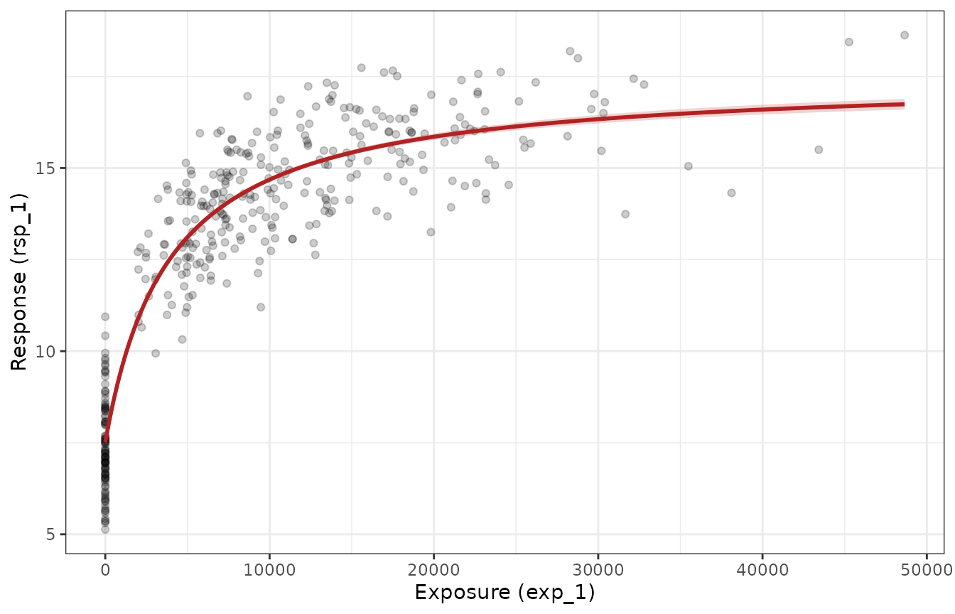

The solid line is the estimated mean response and the shaded band is the pointwise confidence band for that mean. Use interval = "prediction" instead if you want an interval for a new observation rather than for the mean.

If you need the underlying prediction function itself — for instance to evaluate the curve at arbitrary parameter values — emax_fun() extracts it from the fitted object.

Comparing models

Adding a covariate defines a nested pair of models, which can be compared. Here we fit a baseline model with no covariates and compare it to the model above.

mod_0 <- emax_nls(
  structural_model = rsp_1 ~ exp_1,
  covariate_model = list(E0 ~ 1, Emax ~ 1, logEC50 ~ 1),
  data = emax_df
)

# information criteria: lower is better
AIC(mod_0, mod)
#>       df    AIC
#> mod_0  4 1281.1
#> mod    5  603.6

# likelihood-ratio style comparison of the nested models
anova(mod_0, mod)
#> Analysis of Variance Table
#> 
#> Model 1: rsp_1 ~ ((1 * E0_Intercept)) + exp_1 * ((1 * Emax_Intercept))/(exp_1 + exp((1 * logEC50_Intercept)))
#> Model 2: rsp_1 ~ ((cnt_a * E0_cnt_a) + (1 * E0_Intercept)) + exp_1 * ((1 * Emax_Intercept))/(exp_1 + exp((1 * logEC50_Intercept)))
#>   Res.Df Res.Sum Sq Df Sum Sq F value Pr(>F)    
#> 1    397        565                             
#> 2    396        103  1    461    1769 <2e-16 ***
#> ---
#> Signif. codes:  0 '***' 0.001 '**' 0.01 '*' 0.05 '.' 0.1 ' ' 1

Because cnt_a genuinely affects the response, the richer model should have the lower AIC and the anova() comparison should favour it. BIC() is available too and applies a heavier penalty per parameter.

A sigmoidal example

To fit a sigmoidal model, add a logHill term to the covariate model. Here we estimate a single Hill coefficient with no covariates on it:

mod_sig <- emax_nls(
  structural_model = rsp_1 ~ exp_1,
  covariate_model = list(E0 ~ cnt_a, Emax ~ 1, logEC50 ~ 1, logHill ~ 1),
  data = emax_df
)
coef(mod_sig, back_transform = TRUE)
#>       E0_cnt_a   E0_Intercept Emax_Intercept EC50_Intercept Hill_Intercept 
#>         0.4864         5.0544         9.9068      3866.1810         1.0173

The data were generated with a Hill coefficient of $1$ , so the back-transformed Hill_Intercept should sit near $1$ and the sigmoidal model should offer little improvement over the hyperbolic one — which is exactly the kind of check AIC() is for:

AIC(mod, mod_sig)
#>         df   AIC
#> mod      5 603.6
#> mod_sig  6 605.6

Where to go next

This article covered the mechanics of fitting and interpreting a single continuous-outcome Emax model. From here you might look at:

Covariate selection. When there are many candidate covariates, emax_scm_forward() and emax_scm_backward() automate stepwise addition and elimination, and emax_scm_history() records every model that was tried.
Simulation. The simulate() method draws new response datasets from the fitted model while propagating parameter uncertainty, which is useful for predictive checks and simulation-based confidence bands.
Binary outcomes. For 0/1 responses, use emax_logistic(), which places the Emax model on the logit scale and estimates it by iterative reweighted least squares. It is described in its own article.