Fitting Emax models for binary outcomes

library(emaxnls)
library(tibble)
library(ggplot2)
theme_set(theme_bw())
set.seed(123)

This article describes how to fit an Emax regression model to a binary (0/1) outcome with emax_logistic(). It is the companion to the article on continuous outcomes, and the interface is deliberately parallel: you specify a structural_model, a covariate_model, and data in exactly the same way. The statistical machinery underneath is different, though, because a binary response cannot be modelled with ordinary least squares. This article focuses on those differences — the logit link, the Bernoulli error model, and why estimation uses iterative reweighted least squares (IRLS) rather than a single call to nls().

If you have not already read the continuous-outcome article, it is worth skimming first: the meaning of the structural parameters ( $E_0$ , $E_{\max}$ , $EC_{50}$ , and the optional Hill coefficient) and the way covariates enter as linear submodels are shared between the two model types and are not repeated in full here.

The model

A structural model on the logit scale

For a binary outcome we model the probability of a positive response, $p = \Pr(Y = 1)$ , as a function of exposure. Probabilities are confined to the interval $(0, 1)$ , but the Emax structural form is unbounded, so we do not model $p$ directly. Instead the Emax model is placed on the log-odds (logit) scale:

$\operatorname{logit}(p) = \log\!\left(\frac{p}{1 - p}\right) = E_0 + E_{\max}\,\frac{x}{x + EC_{50}},$

with the sigmoidal (Hill) version

$\operatorname{logit}(p) = E_0 + E_{\max}\,\frac{x^{h}}{x^{h} + EC_{50}^{\,h}}$

available by adding a logHill term to the covariate model, exactly as in the continuous case. The structural parameters have the same roles as before, but they now live on the logit scale: $E_0$ is the baseline log-odds at zero exposure, and $E_{\max}$ is the maximal change in log-odds that the drug can produce. As before, $EC_{50}$ and the Hill coefficient are estimated on the log scale as logEC50 and logHill, and each structural parameter can carry its own covariates.

The logit link is what connects this unbounded linear-on-the-logit-scale predictor back to a probability. Writing $\eta$ for the right-hand side (the linear predictor), the mean response is recovered through the inverse-logit (logistic) function

$p = \operatorname{logit}^{-1}(\eta) = \frac{1}{1 + e^{-\eta}},$

which maps any real value of $\eta$ into $(0, 1)$ . This guarantees that fitted and predicted probabilities are always valid, no matter what values the structural parameters take.

The Bernoulli error model

Once the mean $p_i$ for observation $i$ is specified, we still need an assumption about how the observed 0/1 outcomes scatter around it. For binary data the natural choice is the Bernoulli distribution:

$Y_i \sim \operatorname{Bernoulli}(p_i), \qquad \Pr(Y_i = y_i) = p_i^{\,y_i}\,(1 - p_i)^{1 - y_i}.$

Two consequences of this error model matter for estimation. First, the likelihood we want to maximise is the Bernoulli (log-)likelihood

$\ell(\theta) = \sum_{i=1}^{n}\Big[\, y_i \log p_i + (1 - y_i)\log(1 - p_i)\,\Big],$

which is what logLik() returns and what deviance() reports as $-2\ell(\theta)$ (the binomial deviance). Second, the variance of a Bernoulli observation is $\operatorname{Var}(Y_i) = p_i(1 - p_i)$ : it is not constant, but depends on the mean. Observations with $p_i$ near $0$ or $1$ are far more informative than those near $0.5$ . This mean-variance link is precisely what ordinary least squares ignores, and it is the reason a bare nls() fit is inappropriate here.

Why not a bare call to `nls()`?

It is tempting to just fit the structural Emax curve to the 0/1 responses with nls(), minimising $\sum_i (y_i - p_i)^2$ . This is a bad idea for several related reasons:

The wrong error model. Least squares is the maximum-likelihood estimator only under Gaussian errors with constant variance. Binary data have variance $p_i(1 - p_i)$ , which changes with the mean. Treating every observation as equally precise gives statistically inefficient estimates and, more seriously, standard errors, confidence intervals, and $p$ -values that are simply wrong.
Unbounded predictions. Fitting the Emax form directly on the probability scale places no constraint on $p_i$ , so nothing stops the fitted curve from drifting below $0$ or above $1$ . The logit link removes this problem by construction.
Not the maximum-likelihood estimate. Minimising squared error does not maximise the Bernoulli likelihood, so the resulting estimates lack the consistency and efficiency properties we rely on for inference.

The standard remedy for generalised linear models is iterative reweighted least squares (IRLS), also known as Fisher scoring. The idea is to replace the single least-squares problem with a sequence of weighted least-squares problems that progressively account for the mean-variance relationship. At each iteration, given the current linear predictor $\eta$ and fitted probabilities $\mu = \operatorname{logit}^{-1}(\eta)$ , we form

$w_i = \mu_i(1 - \mu_i) \qquad\text{(working weights)}, \qquad z_i = \eta_i + \frac{y_i - \mu_i}{w_i} \qquad\text{(working response)},$

and solve a weighted least-squares fit of the working response $z$ on the structural model, using weights $w$ . The weights are exactly the Bernoulli variance function, so more informative observations are up-weighted; the working response is a local linearisation of the link. Iterating this scheme is equivalent to Fisher scoring and converges to the maximum-likelihood estimates under the Bernoulli model.

There is one extra wrinkle specific to Emax models. In an ordinary logistic linear regression each weighted step is a linear least-squares problem. Here the structural predictor is nonlinear in the parameters (exposure enters through $x/(x + EC_{50})$ ), so each weighted step is itself a weighted nonlinear least squares problem. emax_logistic() therefore layers the IRLS loop on top of nls(): the inner weighted NLS solve reuses the same three optimisation algorithms available for continuous models ("gauss", "port", "levenberg"), while the outer loop updates the weights and working response. The loop is initialised in the GLM-standard way (starting from $\mu = (y + 1/2)/2$ to avoid degenerate weights at $0$ and $1$ ), warm-starts each NLS solve from the previous estimates, and stops when the change in binomial deviance falls below a tolerance. Both the tolerance and the maximum number of outer iterations are controlled by emax_logistic_options():

emax_logistic_options()
#> $optim_method
#> [1] "gauss"
#> 
#> $optim_control
#> $optim_control$maxiter
#> [1] 50
#> 
#> $optim_control$tol
#> [1] 1e-05
#> 
#> $optim_control$minFactor
#> [1] 0.0009766
#> 
#> $optim_control$printEval
#> [1] FALSE
#> 
#> $optim_control$warnOnly
#> [1] FALSE
#> 
#> $optim_control$scaleOffset
#> [1] 0
#> 
#> $optim_control$nDcentral
#> [1] FALSE
#> 
#> 
#> $quiet
#> [1] FALSE
#> 
#> $weights
#> NULL
#> 
#> $na.action
#> function (object, ...) 
#> UseMethod("na.omit")
#> <bytecode: 0x558ce5176288>
#> <environment: namespace:stats>
#> 
#> $max_iter
#> [1] 25
#> 
#> $tol
#> [1] 1e-06
#> 
#> $max_time
#> [1] Inf

The example data

We again use the bundled synthetic dataset emax_df, this time focusing on the binary response rsp_2.

emax_df
#> # A tibble: 400 × 12
#>       id  dose  exp_1  exp_2 rsp_1 rsp_2 cnt_a cnt_b cnt_c bin_d bin_e cat_f
#>    <int> <dbl>  <dbl>  <dbl> <dbl> <dbl> <dbl> <dbl> <dbl> <dbl> <dbl> <fct>
#>  1     1   200 12332. 13004. 15.7      1  3.85  5.89  4.31     1     1 grp 1
#>  2     2   300 18232. 17244. 15.3      1  4.78  7.25  3.73     1     1 grp 1
#>  3     3     0     0      0   5.65     0  1.22  9.24  2.41     1     1 grp 1
#>  4     4   200  9394.  8839. 12.5      0  2.68  7.14  3.76     1     1 grp 2
#>  5     5   200  7088.  9827. 13.2      1  4.27  5.57  9.05     0     1 grp 2
#>  6     6   300 30402. 28483. 16.8      1  6.09  6.08  4.62     0     1 grp 1
#>  7     7   300 21679. 17137. 17.4      1  7.5   8.1   2.08     0     1 grp 3
#>  8     8   100 15506. 13377. 15.9      0  3.65  6.89  3.56     0     1 grp 1
#>  9     9     0     0      0   7.3      0  4.84  3.77  7.44     0     1 grp 2
#> 10    10   200  5331.  5251. 12.8      1  4.45  3.42  1.66     1     0 grp 3
#> # ℹ 390 more rows

The binary response was generated from a logit-scale Emax model with $E_0 = -4.5$ , $E_{\max} = 5$ , and $EC_{50} = 8000$ ( $\log EC_{50} \approx 8.99$ ), plus genuine covariate effects of cnt_a (coefficient $0.5$ ) and bin_d (coefficient $1$ ) on the baseline; the remaining covariates have no effect. In other words the data-generating linear predictor is

$\operatorname{logit}(p) = -4.5 + 5\,\frac{x}{x + 8000} + 0.5\,\texttt{cnt\_a} + 1.0\,\texttt{bin\_d}.$

Binary outcomes carry much less information per observation than continuous ones, so we should expect the structural parameters — especially $E_{\max}$ and $EC_{50}$ — to be estimated with considerably more uncertainty than in the continuous article.

Fitting the model

The call mirrors emax_nls() exactly. We start with a deliberately simple covariate model that puts only cnt_a on the baseline, and add bin_d later.

mod <- emax_logistic(
  structural_model = rsp_2 ~ exp_1,
  covariate_model = list(
    E0 ~ cnt_a,   # baseline log-odds depends on cnt_a
    Emax ~ 1,
    logEC50 ~ 1
  ),
  data = emax_df
)

As always, check convergence before interpreting anything. For an emaxlogistic model this means both that the inner NLS solves succeeded and that the outer IRLS loop reached its deviance tolerance.

emax_converged(mod)
#> [1] TRUE

Printing the object reports the structural and covariate models, notes that the response is binary with a logit link, and summarises the fit with the number of observations, the residual degrees of freedom, the binomial deviance, and the AIC, followed by a coefficient table with confidence intervals.

mod
#> Structural model:
#> 
#>   Exposure:       exp_1 
#>   Response:       rsp_2 
#>   Emax type:      hyperbolic 
#>   Response type:  binary (logit link)
#> 
#> Covariate model:
#> 
#>   E0:       E0 ~ cnt_a 
#>   Emax:     Emax ~ 1 
#>   logEC50:  logEC50 ~ 1 
#> 
#> Model fit:
#> 
#>   Observations:  400 
#>   Residual df:   396 
#>   Deviance:      331.5 
#>   AIC:           339.5 
#> 
#> Coefficients (95% CI):
#> 
#>   label             estimate std_error  lower  upper
#> 1 E0_cnt_a             0.659    0.0800  0.501  0.816
#> 2 E0_Intercept        -5.00     0.578  -6.14  -3.87 
#> 3 Emax_Intercept       8.12     2.27    5.08  17.6  
#> 4 logEC50_Intercept    9.78     0.518   8.89  11.0  
#> 
#> Use summary() for hypothesis tests.

Interpreting the output

Coefficients are on the logit scale

coef() returns the estimates. Because the structural model lives on the logit scale, every coefficient is interpreted there: E0_Intercept is the baseline log-odds, E0_cnt_a is the change in baseline log-odds per unit of cnt_a, and so on.

coef(mod)
#>          E0_cnt_a      E0_Intercept    Emax_Intercept logEC50_Intercept 
#>            0.6588           -5.0004            8.1157            9.7832

A one-unit increase in cnt_a multiplies the odds of a positive response by $e^{0.66} \approx 1.93$ — exponentiating a logit-scale coefficient turns it into an odds ratio, the usual way to report effects from a logistic model. As in the continuous case, back_transform = TRUE exponentiates the log-scale structural parameters (logEC50, and logHill if present), returning EC50/Hill on their natural scales:

coef(mod, back_transform = TRUE)
#>       E0_cnt_a   E0_Intercept Emax_Intercept EC50_Intercept 
#>         0.6588        -5.0004         8.1157     17733.7870

The estimated baseline (E0_Intercept near the true $-4.5$ ) and the cnt_a effect (near the true $0.5$ ) are recovered reasonably well, whereas the structural $E_{\max}$ and $EC_{50}$ are less precisely pinned down — a direct consequence of how little information binary observations carry about the shape of the exposure-response curve.

Standard errors, tests, and confidence intervals

summary() gives the coefficient table. Note that the test statistic is a z-statistic (a Wald test referred to the standard normal distribution), reflecting the asymptotic-normal justification for inference in a maximum-likelihood GLM, rather than the $t$ -statistic used for continuous models.

summary(mod)
#> # A tibble: 4 × 7
#>   label             estimate std_error z_statistic   p_value ci_lower ci_upper
#>   <chr>                <dbl>     <dbl>       <dbl>     <dbl>    <dbl>    <dbl>
#> 1 E0_cnt_a             0.659    0.0800        8.24  1.79e-16    0.501    0.816
#> 2 E0_Intercept        -5.00     0.578        -8.64  5.43e-18   -6.14    -3.87 
#> 3 Emax_Intercept       8.12     2.27          3.58  3.45e- 4    5.08    17.6  
#> 4 logEC50_Intercept    9.78     0.518        NA    NA           8.89    11.0

confint() computes profile-likelihood intervals from the final weighted NLS fit at convergence. These are especially valuable here: for weakly identified parameters such as Emax_Intercept and logEC50_Intercept the likelihood is distinctly non-quadratic, so the profile intervals are wide and asymmetric in a way that a symmetric Wald interval would misrepresent.

confint(mod)
#>                      2.5%  97.5%
#> E0_cnt_a           0.5015  0.816
#> E0_Intercept      -6.1358 -3.867
#> Emax_Intercept     5.0801 17.608
#> logEC50_Intercept  8.8921 11.048

Note that there is no sigma() method for a logistic model: the Bernoulli variance is fixed by the mean through $p(1 - p)$ , so there is no free residual standard-deviation parameter to estimate.

Fitted values, residuals, and predictions

fitted() returns fitted probabilities by default, or the linear predictor on the logit scale with type = "link":

head(fitted(mod))
#> [1] 0.70364 0.90573 0.01482 0.39544 0.53245 0.98428
head(fitted(mod, type = "link"))
#> [1]  0.8647  2.2626 -4.1967 -0.4245  0.1300  4.1373

Raw residuals are not very informative for binary data, so residuals() returns Pearson residuals by default (raw residual divided by $\sqrt{\mu(1-\mu)}$ ) and deviance residuals on request (whose sum of squares equals the model deviance):

head(residuals(mod))                    # Pearson
#> [1]  0.6490  0.3226 -0.1227 -0.8088  0.9371  0.1264
head(residuals(mod, type = "deviance")) # deviance
#> [1]  0.8384  0.4450 -0.1728 -1.0033  1.1227  0.1780

predict() behaves like its continuous counterpart but is link-aware. By default it returns probabilities; with type = "link" it returns the linear predictor. When an interval is requested, the bounds are computed on the logit scale and then passed through the inverse-logit transformation, so they are guaranteed to stay within $(0, 1)$ on the probability scale. We use this to draw the fitted probability curve over a grid of exposures, holding cnt_a at its mean:

grid <- tibble(
  exp_1 = seq(0, max(emax_df$exp_1), length.out = 200),
  cnt_a = mean(emax_df$cnt_a)
)
pred <- predict(mod, newdata = grid, interval = "confidence")
curve <- tibble(
  exp_1 = grid$exp_1,
  fit = pred[["fit"]],
  lwr = pred[["lwr"]],
  upr = pred[["upr"]]
)

ggplot(mapping = aes(exp_1)) +
  geom_jitter(
    aes(y = rsp_2),
    data = emax_df,
    height = 0.03,
    width = 0,
    alpha = 0.2
  ) +
  geom_ribbon(
    aes(ymin = lwr, ymax = upr),
    data = curve,
    fill = "steelblue",
    alpha = 0.2
  ) +
  geom_line(aes(y = fit), data = curve, colour = "steelblue", linewidth = 1) +
  labs(x = "Exposure (exp_1)", y = "P(rsp_2 = 1)")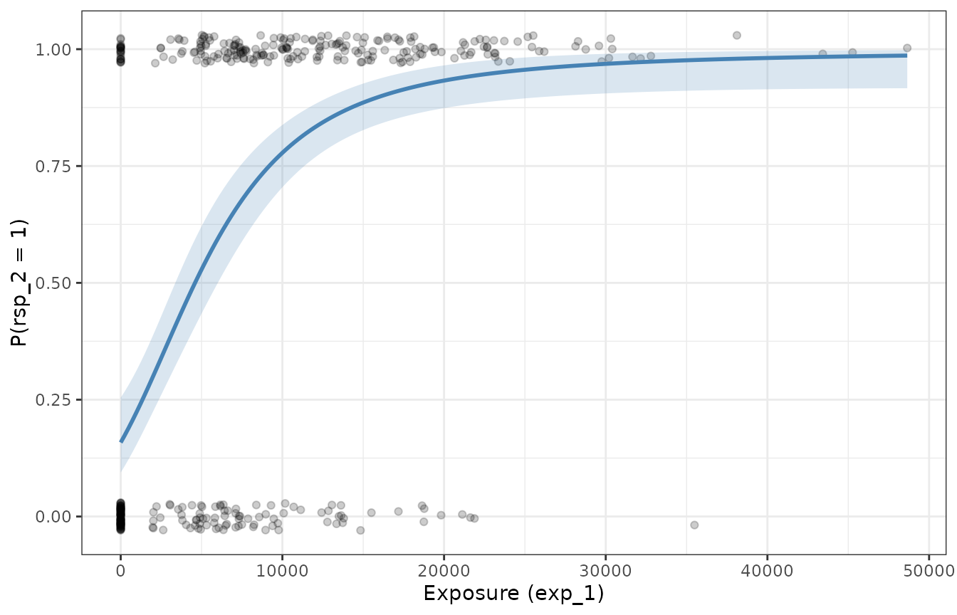

The raw 0/1 outcomes are jittered vertically so they can be seen; the solid line is the estimated probability of a positive response as a function of exposure, and the shaded band is its pointwise confidence band.

Comparing models

Model comparison uses the Bernoulli likelihood. AIC() (and BIC()) are built from the binomial deviance plus a penalty per parameter, and anova() performs a likelihood-ratio test: the test statistic is the drop in deviance between nested models, referred to a chi-squared distribution with degrees of freedom equal to the difference in the number of parameters.

Recall that bin_d has a genuine effect in the data-generating model but was omitted above. Adding it should improve the fit substantially:

mod_bin_d <- emax_logistic(
  structural_model = rsp_2 ~ exp_1,
  covariate_model = list(E0 ~ cnt_a + bin_d, Emax ~ 1, logEC50 ~ 1),
  data = emax_df
)

# information criterion: lower is better
AIC(mod, mod_bin_d)
#>           df   AIC
#> mod        4 339.5
#> mod_bin_d  5 326.0

# likelihood-ratio test for the added covariate
anova(mod, mod_bin_d)
#>      Df Deviance Df_diff  LRT Pr(>Chi)    
#> [1,]  4      331                          
#> [2,]  5      316       1 15.4  8.5e-05 ***
#> ---
#> Signif. codes:  0 '***' 0.001 '**' 0.01 '*' 0.05 '.' 0.1 ' ' 1

The richer model has the lower AIC and the likelihood-ratio test strongly favours it, and the estimated E0_bin_d coefficient lands near the true value of $1$ :

coef(mod_bin_d)
#>          E0_cnt_a          E0_bin_d      E0_Intercept    Emax_Intercept 
#>            0.6926            1.1114           -5.6865            7.9922 
#> logEC50_Intercept 
#>            9.7520

Where to go next

The remaining tools work for emaxlogistic objects just as they do for continuous models:

Covariate selection. emax_scm_forward() and emax_scm_backward() run stepwise selection using the same p-value criterion, and emax_scm_history() records every model tried.
Simulation. The simulate() method draws parameter values from their estimated distribution, computes the implied probabilities, and then draws fresh Bernoulli outcomes — useful for predictive checks and simulation-based intervals.
Continuous outcomes. For a continuous response, use emax_nls(), described in its own article.